The {sherlock} R package provides powerful graphical displays and statistical tools to aid structured problem solving and diagnosis. The functions of the package are especially useful for applying the process of elimination as a problem diagnosis technique. {sherlock} was designed to seamlessly work with the tidyverse set of packages.
More specifically, {sherlock} features functionality to
- create a project folder/sub-folder structure and .Rproj file for your problem solving project with one function call
- read in tabular data from various sources
- facilitate reading in and cleaning many files all at once (for example raw data from data loggers or sensors)
- create powerful and highly customizable visual displays, some of which are non-existent even in popular statistical packages
- use a custom {sherlock} ggplot2 theme, which offers a clean-looking visual appearance
- use sample datasets to test plotting functions
- save data and plots into an Excel file
“That is to say, nature’s laws are causal; they reveal themselves by comparison and difference, and they operate at every multi-variate space-time point” - Edward Tufte
I would love to hear your feedback on sherlock. You can leave a note on current issues, bugs and even request new features here.
sherlock 0.6.0 is now released. In addition to fixing a few bugs and making enhancements to already-existing functionality, new plotting, statistical analysis and helper functions have been added, such as:
- A new set of plotting functions and statistical tests called the Tukey-Duckworth test for problem diagnosis. These are
plot_tukey_duckworth_test()andplot_tukey_duckworth_paired_test(). -
select_low_high_units()andselect_low_high_units_manual(): Automatically or manually select low-high units in a tibble as well as assign them into groups. -
load_files(), which is a function to read in and clean multiple files. Particularly useful when reading in multiple files having the same variables, for example reading in data from an experiment where data was logged and saved separately for each individual unit. Integration of a custom data cleaning function. -
create_project_folder(), which is a helper function to quickly create a project folder with a clever sub-folder structure for your project.
Installation
sherlock is available on CRAN and can be installed by running the below script:
install.packages("sherlock")You can also install the development version of sherlock from GitHub with:
# install.packages("devtools")
devtools::install_github("gaborszabo11/sherlock")
Functions
Examples
Here are a few examples:
# Loading libraries
library(sherlock)
library(ggh4x)
#> Loading required package: ggplot2
#> Warning: package 'ggplot2' was built under R version 4.2.2
multi_vari_data %>%
  draw_multivari_plot(y_var = force,
                      grouping_var_1 = cycle,
                      grouping_var_2 = fixture,
                      grouping_var_3 = line)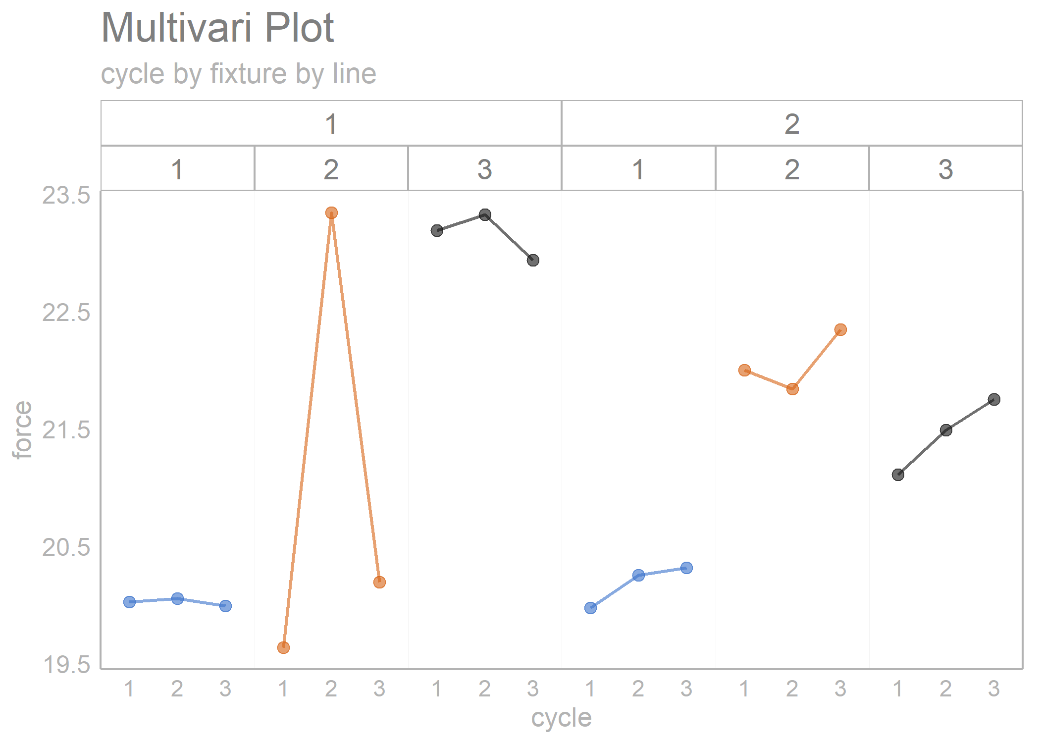
library(sherlock)
library(ggh4x)

multi_vari_data_2 %>%
  draw_multivari_plot(y_var = Length,
                      grouping_var_1 = Part,
                      grouping_var_2 = Operator, plot_means = TRUE)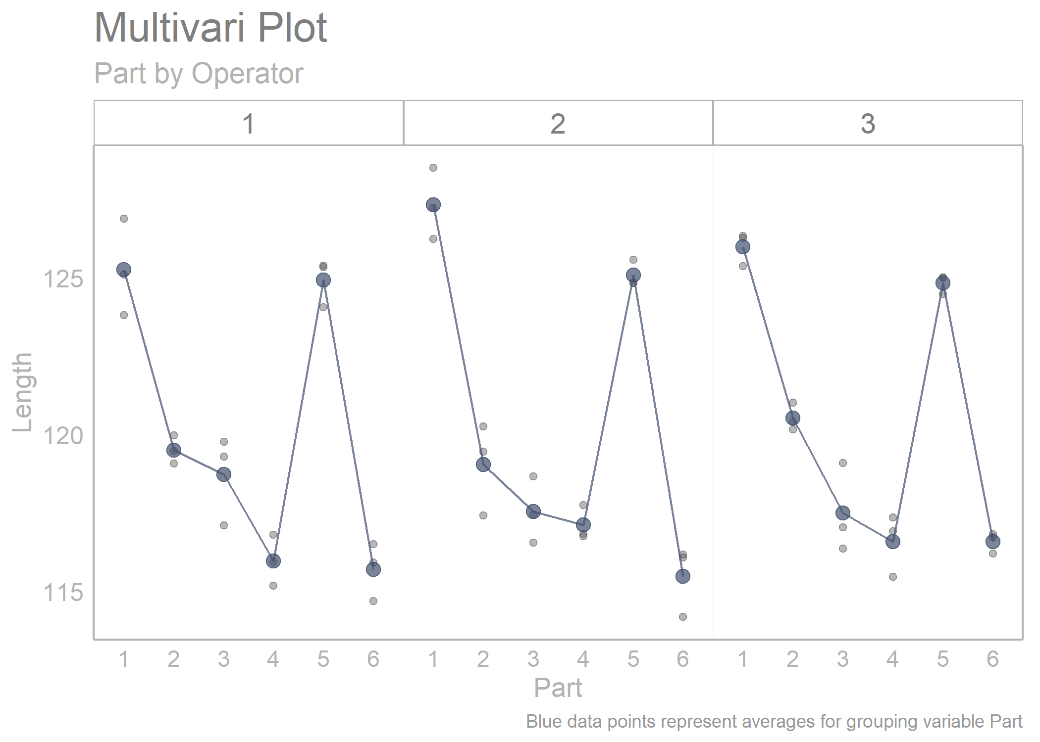
library(sherlock)
library(dplyr)
#>
#> Attaching package: 'dplyr'
#> The following objects are masked from 'package:stats':
#>
#>     filter, lag
#> The following objects are masked from 'package:base':
#>
#>     intersect, setdiff, setequal, union

polar_small_multiples_data %>%
  filter(Mold_Cavity_Number %in% c(4, 6)) %>%
  rename(Radius = "ID_2") %>%
  draw_polar_small_multiples(angular_axis   = ID_Measurement_Angle,
                             x_y_coord_axis = Radius,
                             grouping_var   = Tip_Bottom,
                             faceting_var_1 = Mold_Cavity_Number,
                             point_size     = 0.5,
                             connect_with_lines = TRUE,
                             label_text_size = 7) +
  scale_y_continuous(limits = c(0.09, 0.115))
#> Scale for y is already present.
#> Adding another scale for y, which will replace the existing scale.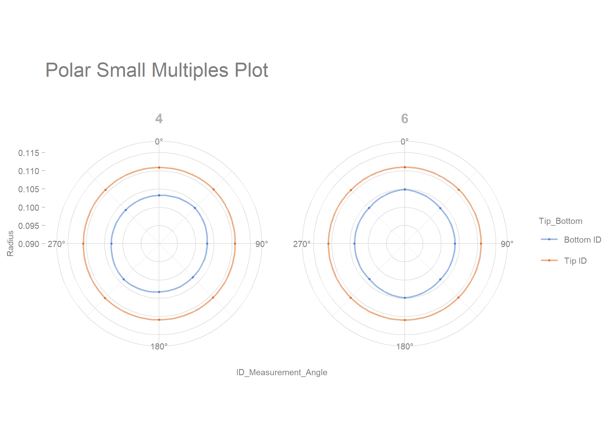
library(sherlock)
library(dplyr)
library(ggh4x)

polar_small_multiples_data %>%
  filter(ID_Measurement_Angle %in% c(0, 45, 90, 135)) %>%
  normalize_observations(y_var = ID, grouping_var = Tip_Bottom, ref_values = c(0.2075, 0.2225)) %>%
  draw_multivari_plot(y_var             = ID_normalized,
                      grouping_var_1    = ID_Measurement_Angle,
                      grouping_var_2    = Mold_Cavity_Number,
                      grouping_var_3    = Tip_Bottom,
                      x_axis_text = 6) +
  draw_horizontal_reference_line(reference_line = 0)
#> Joining, by = "Tip_Bottom"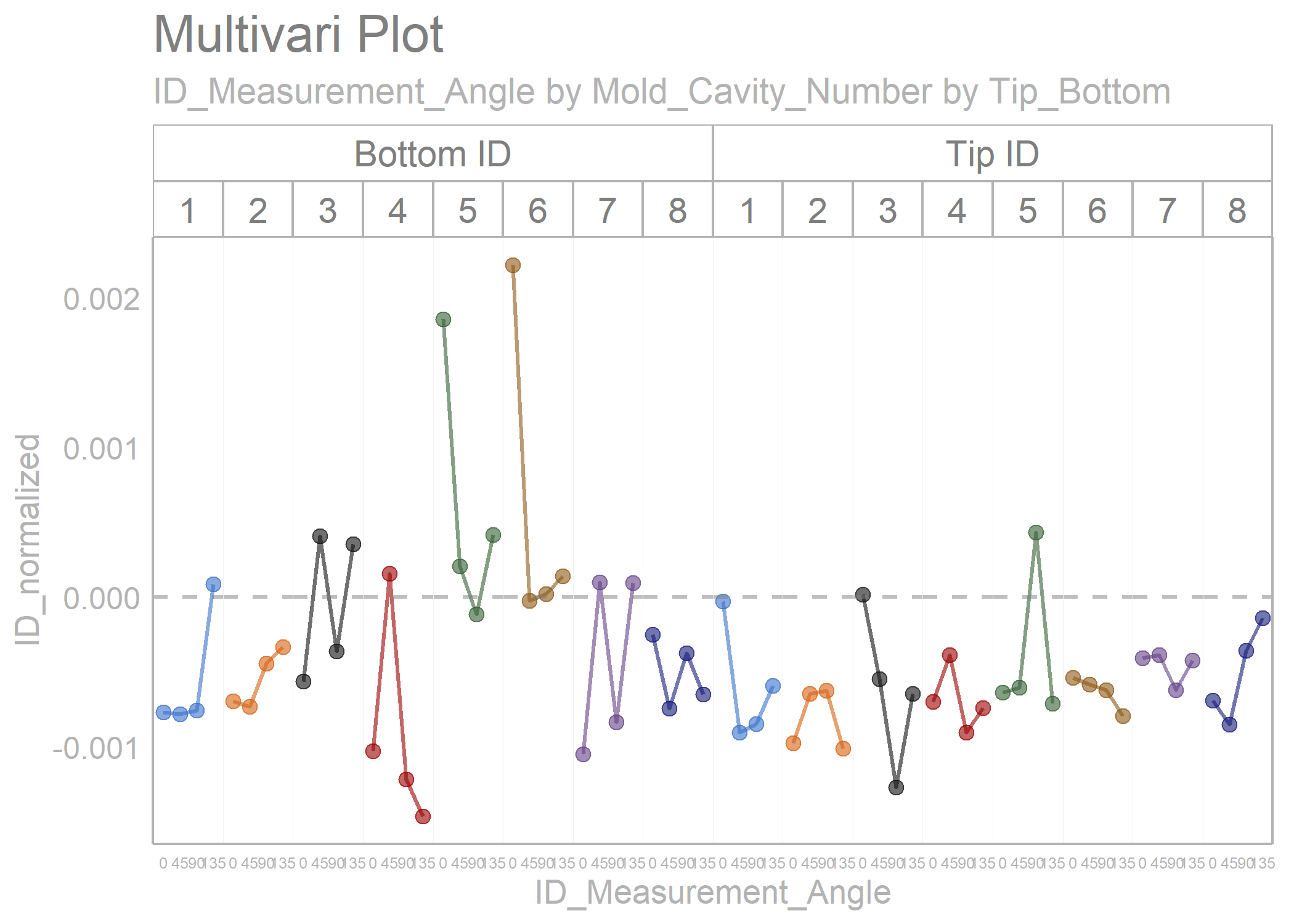
youden_plot_data_2 %>%
  draw_youden_plot(x_axis_var  = gage_1,
                   y_axis_var  = gage_2,
                   median_line = TRUE)
#> Smoothing formula not specified. Using: y ~ x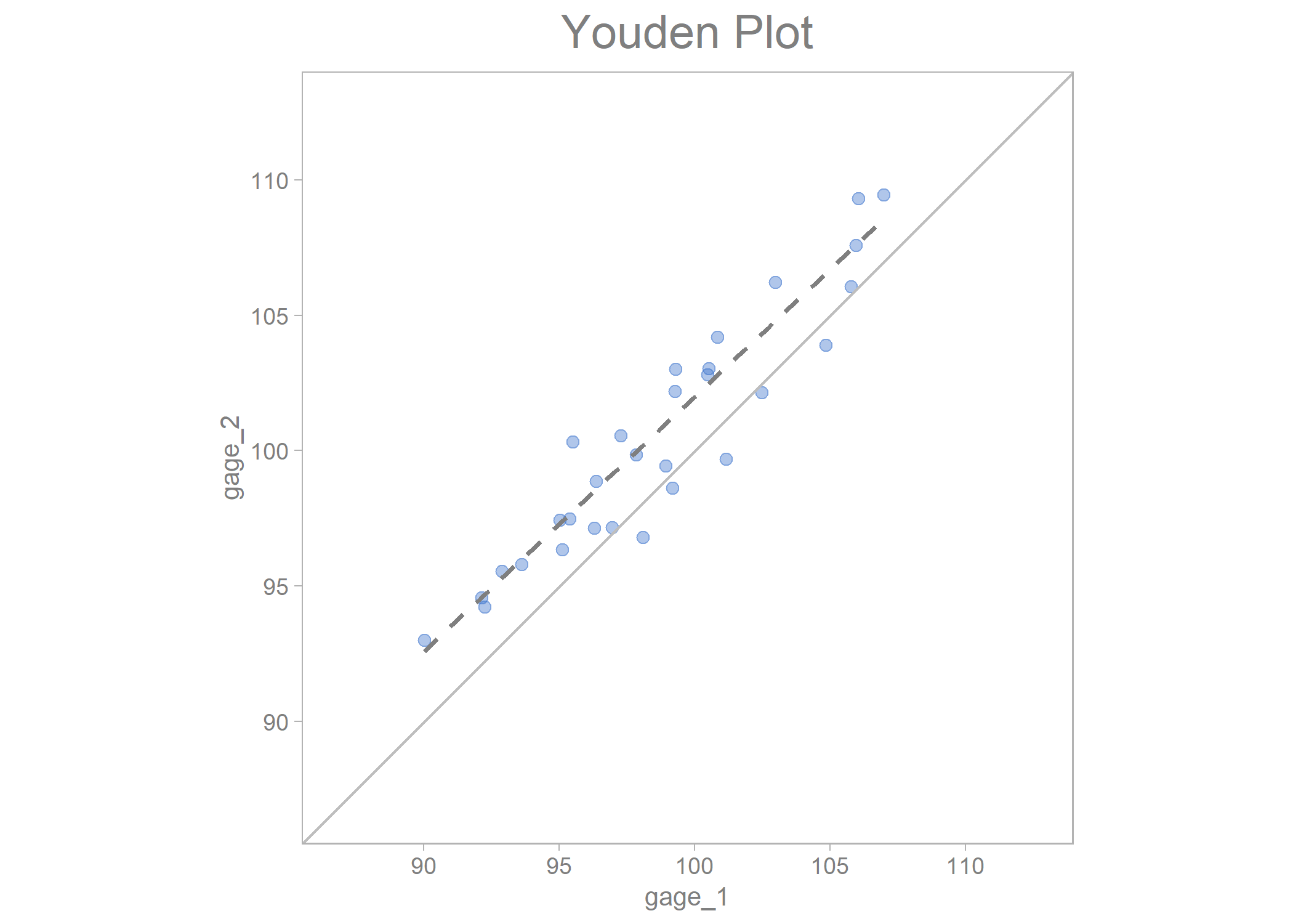
youden_plot_data %>%
  draw_youden_plot(x_axis_var   = measurement_1,
                   y_axis_var   = measurement_2,
                   grouping_var = location,
                   x_axis_label = "Trial 1",
                   y_axis_label = "Trial 2")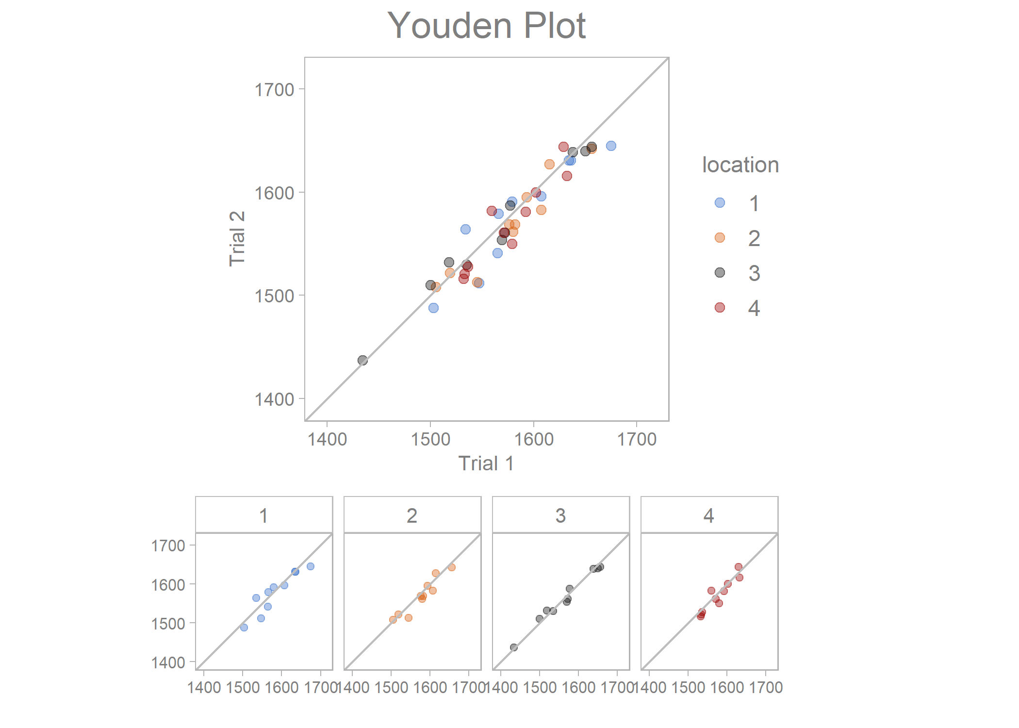
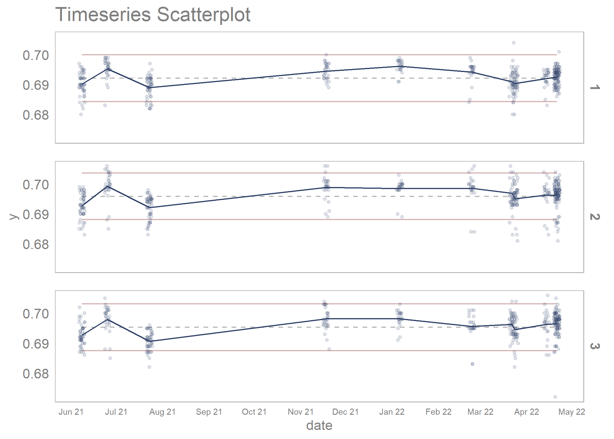
timeseries_scatterplot_data %>%
  draw_timeseries_scatterplot(y_var = y,
                              grouping_var_1 = date,
                              grouping_var_2 = cavity,
                              faceting       = TRUE,
                              limits         = TRUE,
                              alpha          = 0.15,
                              line_size      = 0.5,
                              x_axis_text    = 7,
                              interactive    = FALSE)
#> Joining, by = c("date", "cavity")
#> Warning: Removed 6 rows containing missing values (`geom_point()`).